<-- Back to Previous Page	TOC	Next Chapter -->

Chapter 1: The Digital Representation of Sound,
Part One: Sound and Timbre

Section 1.4: Timbre

What’s the difference between a tuba and a flute (or, more accurately, the sounds of each)? How do we tell the difference between two people singing the same song, when they’re singing exactly the same notes? Why do some guitars "sound" better than others (besides the fact that they’re older or cost more or have Eric Clapton’s autograph on them)? What is it that makes things "sound" like themselves?

It’s not necessarily the pitch of the sound (how high or low it is)—if everyone in your family sang the same note, you could almost surely tell who was who, even with your eyes closed. It’s also not just the loudness—your voice is still your voice whether you talk softly or scream at the top of your lungs. So what’s left? The answer is found in a somewhat mysterious and elusive thing we call, for lack of a better word, "timbre," and that’s what this section is all about.

"Timbre" (pronounced "tam-ber") is a kind of sloppy word, inherited from previous eras, that lumps together lots of things that we don’t fully understand. Some think we should abandon the word and concept entirely! But it’s one of those words that gets used a lot, even if it doesn’t make much sense, so we’ll use it here too—we’re sort of stuck with it for the time being.

Applet 1.9
Draw a waveform

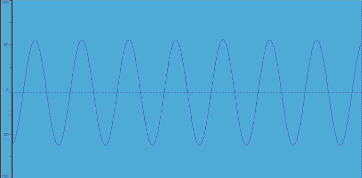
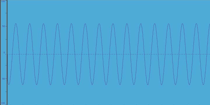
This applet lets you draw a periodic waveform. How much does the shape of the waveform (which is a result of its steady-state spectra) influence what you hear? Some shapes seem to sound "brighter" than others, some "duller."

We’ll see, as we learn more about timbre, that the periodic waveform shape may not be all that important when it comes to our recognizing, distinguishing, and identifying sounds. This is somewhat surprising, and contrary to 100 years of popular assumption. But you may notice, after all, that in redrawing the waveform you might not feel that you’re creating a whole new sound event, just a kind of different "buzz."

What Makes Up Timbre?

Timbre can be roughly defined as those qualities of a sound that aren’t just frequency or amplitude. These qualities might include:

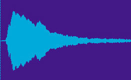
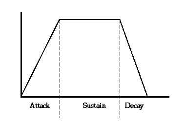
spectra: the aggregate of simpler waveforms (usually sine waves) that make up what we recognize as a particular sound. This is what Fourier analysis gives us (we’ll discuss that in Chapter 3).
envelope: the attack, sustain, and decay portions of a sound (often referred to as transients).

Envelope and spectra are very complicated concepts, encompassing a lot of subcategories. For example, spectral features are very important, different ways that the spectral aggregates are organized statistically in terms of shape and form (e.g., the relative "noisiness" of a sound is a result, in large part, of its spectral relationships). Many facets of envelope (onset time, harmonic decay, spectral evolution, steady-state modulations, etc.) are not easily explained by just looking at the envelope of a sound. Researchers spend a great deal of time on very specific aspects of these ideas, and it’s an exciting and interesting area for computer musicians to research.

Figure 1.18 shows a simplified picture of the envelope of a trumpet tone.

Figure 1.18 This image illustrates the attack, sustain, and decay portions of a standard amplitude envelope. This is a very simple, idealized picture, called a trapezoidal envelope. We are not aware of any actual, natural occurrence of this kind of straight-lined sound!

It’s helpful here to bring another descriptive term into our vocabulary: spectrum. Spectrum is defined by a waveform’s distribution of energy at certain frequencies. The combination of spectra (plural of spectrum) and envelope helps us to define the "color" of a sound. Timbre is difficult to talk about, because it’s hard to measure something subjective like the "quality" of a sound. This concept gives music theorists, computer musicians, and psychoacousticians a lot of trouble. However, computers have helped us make great progress in the exploration and understanding of the various components of what’s traditionally been called "timbre."

Basic Elements of Sound

As we’ve shown, the average piece of music can be a pretty complicated function. Nevertheless, it’s possible to think of it as a combination of much simpler sounds (and hence simpler functions)—even simpler than individual instruments. The basic atoms of sound, the sinusoids (sine waves) we talked about in the previous sections, are sometimes called pure tones, like those produced when a tuning fork vibrates. We use the tuning fork to talk about these tones because it is one of the simplest physical vibrating systems.

Although you might think that a discussion of tuning forks belongs more in a discussion of frequency, we’re going to use them to introduce the notion of sinusoids: Fourier components of a sound.

Soundfile 1.16
Tuning fork
at 256 Hz

Soundfile 1.17
Sine wave
at 256 Hz

Xtra bit 1.6
Tuning forks

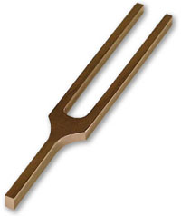
Figure 1.19 This tuning fork rings at 256 Hz. You can hear the sound it makes by clicking on Soundfile 1.16.

Compare the tuning fork sound to that of a pure sine wave at the same frequency of 256 Hz.

When you hit the tines of a tuning fork, it vibrates and emits a very pure note or tone. Tuning forks are able to vibrate at very precise frequencies. The frequency of a tuning fork is the number of times the tip goes back and forth in a second. And this number won’t change, no matter how hard you hit that fork. As we mentioned, the human ear is capable of hearing sounds that vibrate all the way from 20 times a second to 20,000 times a second. Low-frequency sounds are like bass notes, and high-frequency sounds are like treble notes. (Low frequency means that the tines vibrate slowly, and high frequency means that they vibrate quickly.)

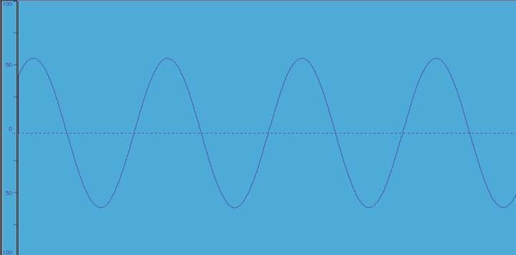
Figure 1.20 Click on the different tuning forks to see the different audiograms. Notice what they have in common! They are all roughly the same shape—simple waves that differ only in the width of the regularly repeating peaks. The higher tones give more peaks over the same interval. In other words, the peaks occur more frequently. (Get it? Higher frequency!)

When you whack the tines of a tuning fork, the fork vibrates. The number of times the tines go back and forth in one second determines the frequency of a particular tuning fork.

Soundfile 1.18
Composer Warren Burt’s piece for tuning forks

Click Soundfile 1.18. You’ll hear composer Warren Burt’s piece for tuning forks, "Improvisation in Two Ancient Greek Modes."

Now, why do tuning fork functions have their simple, sinusoidal shape? Think about how the tip of the tuning fork is moving over time. We see that it is moving back and forth, from its greatest displacement in one direction all the way back to just about the same displacement in the opposite direction.

Imagine that you are sitting on the end of the tine (hold on tight!). When you move to the left, that will be a negative displacement; and when you move to the right, that will be a positive displacement. Once again, as time progresses we can graph the function that at each moment in time outputs your position. Your back-and-forth motion yields the functions many of you remember from trigonometry: sines and cosines.

Figure 1.21 Sine and cosine waves. Thanks to Wayne Mathews for this image.

Any sound can be represented as a combination of different amounts of these sines and cosines of varying frequencies. The mathematical topic that explains sounds and other wave phenomena is called Fourier analysis, named after its discoverer, the great 18th century mathematician Jean Baptiste Joseph Fourier.

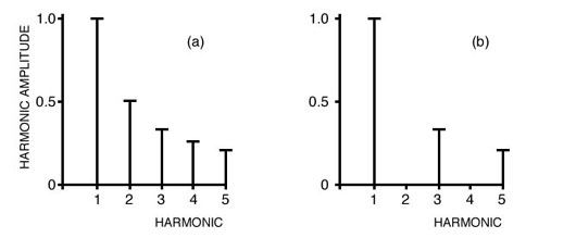
Figure 1.22 Spectra of (a) sawtooth wave and (b) square wave.

Figure 1.22 shows the relative amplitudes of sinusoidal components of simple waveforms.

For example, Figure 1.22(a) indicates that a sawtooth wave can be made by addition in the following way: one part of a sine wave at the fundamental frequency (say, 1 Hz), then half as much of a sine wave at 2 Hz, and a third as much at 3 Hz, and so on, infinitely.

In Section 4.2, we’ll talk about using the Fourier technique in synthesizing sound, called additive synthesis. If you want to jump ahead a bit, try the applet in Section 4.2, that lets you build simple waveforms from sinusoidal components. Notice that when you try to build a square wave, there are little ripples on the edges of the square. This is called Gibbs ringing, and it has to do with the fact that the sum of any finite number of these decreasing amounts of sine waves of increasing frequency is never exactly a square wave.

What the charts in Figure 1.22 mean is that if you add up all those sinusoids whose frequencies are integer multiples of the fundamental frequency of the sound and whose amplitudes are described in the charts by the heights of the bars, you’ll get the sawtooth and square waves.

This is what Fourier analysis is all about: every periodic waveform (which is the same, more or less, as saying every pitched sound) can be expressed as a sum of sines whose frequencies are integer multiples of the fundamental and whose amplitudes are unknown. The sawtooth and square wave charts in Figure 1.22 are called spectral histograms (they don’t show any evolution over time, since these waveforms are periodic).

These sine waves are sometimes referred to as the spectral components, partials, overtones, or harmonics of a sound, and they are what was thought to be primarily responsible for our sense of timbre. So when we refer to the tenth partial of a timbre, we mean a sinusoid at 10 times the frequency of the sound’s fundamental frequency (but we don’t know its amplitude).

The sounds in some of the following soundfiles are conventional instruments with their attacks lopped off, so that we can hear each instrument as a different periodic waveform and listen to each instrument’s different spectral configurations. Notice that, strangely enough, the clarinet (whose sound wave is a lot like a sawtooth wave) and the flute, without their attacks, are not all that different (in the grand scheme of things).

Soundfile 1.19
Clarinet sound

Soundfile 1.20
Clarinet with attack lopped off