Chapter 3: The Frequency Domain

Section 3.3: Fourier and the Sum of Sines

Soundfile 3.5
Adding sine waves

In this section, we’ll try to really explain the notion of a Fourier expansion by building on the ideas of phasors, partials, and sinusoidal components that we introduced in the previous section.

A long time ago, French scientist and mathematician Jean Baptiste Fourier (1768–1830) proved the mathematical fact that any periodic waveform can be expressed as the sum of an infinite set of sine waves. The frequencies of these sine waves must be integer multiples of some fundamental frequency.

In other words, if we have a trumpet sound at middle A (440 Hz), we know by Fourier’s theorem that we can express this sound as a summation of sine waves: 440 Hz, 880Hz, 1,320Hz, 1,760 Hz..., or 1, 2, 3, 4... times the fundamental, each at various amplitudes. This is rather amazing, since it says that for every periodic waveform (one, by the way, that has pitch), we basically know everything about its partials except their amplitudes.

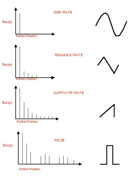
Figure 3.20  The spectrum of the sine wave has energy only at one frequency. The triangle wave has energy at odd-numbered harmonics (meaning odd multiples of the fundamental), with the energy of each harmonic decreasing as 1 over the square of the harmonic number (1/N²). In other words, at the frequency that is N times the fundamental, we have 1/N² as much energy as in the fundamental.

The partials in the sawtooth wave decrease in energy in proportion to the inverse of the harmonic number (1/N). Pulse (or rectangle or square) waveforms have energy over a broad area of the spectrum, but only for a brief period of time.

Fourier Series

What exactly is a Fourier series, and how does it relate to phasors? We use phasors to represent our basic tones. The amazing fact is that any sound can be represented as a combination of phase-shifted, amplitude-modulated tones of differing frequencies. Remember that we got a hint of this concept when we discussed adding phasors in Section 3.2.

A phasor is essentially a way of representing a sinusoidal function. What this means, mathematically, is that any sound can be represented as a sum of sinusoids. This sum is called a Fourier series.

Note that we haven’t limited these sounds to periodic sounds (if we did, we’d have to add that last qualifier about integer multiples of a fundamental frequency). Nonperiodic, or aperiodic, sounds are just as interesting—maybe even more interesting—than periodic ones, but we have to do some special computer tricks to get a nice "harmonic" series out of them for the purposes of analysis and synthesis.

But let’s get down to the nitty-gritty. First, let’s take a look at what happens when we add two sinusoids of the same frequency. Adding a sine and cosine of the same frequency gives a phase-shifted sine of the same frequency:

In fact, the amplitude of the sum, C, is given by:

The phase shift is given by the angle whose tangent is equal to A/B. The shorthand for this is:

We can visualize this with a phasor. Remember that the cosine is just a phase-shifted sine. Since the sine and cosine are moving at the same frequency, they are always "out of sync" by /2, so when we add them it looks like this:

And we get another sinusoid of that frequency.

Any periodic function of period 1 can be written as follows:

We have a nice shorthand for those possibly infinite sums (also called an infinite series):

The two expressions after the Σ signs are called the Fourier coefficients of the function f(t). The Fourier coefficient A₀ has a special name: it is called the DC term, or the DC offset. It tells you the average value of the function. The Fourier coefficients make up a set of numbers called the spectrum of the sound. Now, when you think of the word "spectrum," you might think of colors, like the spectrum of colors of the rainbow. In a way it’s the same: the spectrum tells you how much of each frequency (color) is in the sound.

The values of A_n and B_n for "small" values of n make up the low-frequency information, and we call these the low-order Fourier coefficients. Similarly, the big values of n index the high-frequency information. Since most sounds are made up of a lot of low-frequency information, the low-frequency Fourier coefficients have larger absolute value than the high-frequency Fourier coefficients.

What this means is that it is theoretically possible to take a complex sound, like a person’s voice, and decompose it into a bunch of sine waves, each at a different frequency, amplitude, and phase. These are called the sinusoidal or spectral components of a sound. To find them, we do a Fourier analysis. Fourier synthesis is the inverse process, where we take varying amounts of a bunch of sine waves and add them together (play them at the same time) to reconstruct a sound. Sounds a bit fantastic, doesn’t it? But it works. This process of analyzing or synthesizing a sound based on its component sine waves is called performing a Fourier transform on the sound. When the computer does it, it uses a very efficient technique called the fast Fourier transform (or FFT) for analysis and the inverse FFT (IFFT) for synthesis.

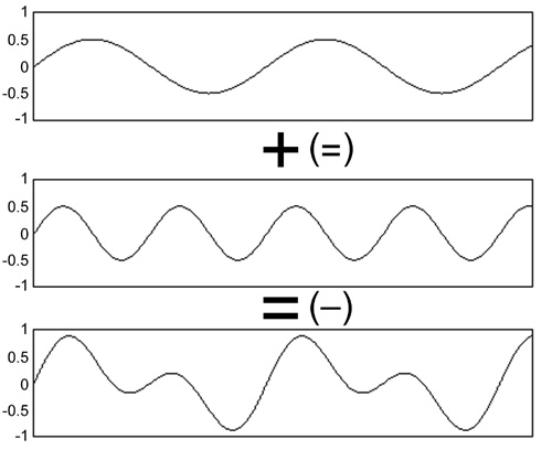
Figure 3.21  What happens if we add a number of sine waves together? We end up with a complicated waveform that is the summation of the individual waves. This picture is a simple example: we just added up two sine waves. For a complex sound, hundreds or even thousands of sine waves are needed to accurately build up the complex waveform. By looking at the illustration from the bottom up, you can see that the inverse is also true—the complex waveform can be broken down into a collection of independent sine waves.

Soundfile 3.6
Trumpet

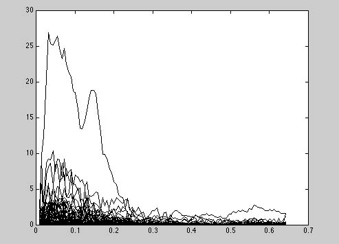
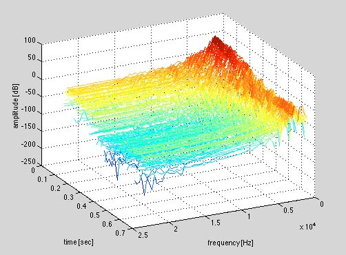
Figure 3.22 A trumpet note in an FFT (fast Fourier transform) analysis—two views. The trumpet sound can be heard by clicking on Soundfile 3.6. Both of these pictures show the evolution of the amplitude of spectral components in time.

The advantage of representing a sound in terms of its Fourier series is that it allows us to manipulate the frequency content directly. If we want to accentuate the high-frequency effects in a sound (make a sound brighter), we could just make all the high-frequency Fourier coefficients bigger in amplitude. If we wanted to turn a sawtooth wave into a square wave, we could just set to zero the Fourier coefficients of the even partials.

Applet 3.3
FFT demo

In fact, we often modify sounds by removing certain frequencies. This corresponds to making a new function where certain Fourier coefficients are set equal to zero while all others are left alone. When we do this we say that we filter the function or sound. These sorts of filters are called bandpass filters, and the frequencies that we leave unaltered in this sort of situation are said to be in the passband. A low-pass filter puts all the low frequencies (up to some bandwidth) in the passband, while a high-pass filter puts all high frequencies (down to some cutoff) in the passband. When we do this, we talk about high-passing and low-passing the sound. In the following soundfiles, we listen to a sound and its high-passed and low-passed versions. We’ll talk a lot more about filters in Chapter 4.

Soundfile 3.7
Filter examples

We start with a sampled file of bugs. This recording was made by composer and sound artist David Dunn using very powerful hydrophones (microphones that work underwater) to amplify the "microsound" of bugs in a pond.

Soundfile 3.8
High-pass filtered

This is David Dunn’s bugs sound file filtered so that we hear only the frequencies above 1,000 Hz. In other words, we have high-pass filtered the sound.

Soundfile 3.9
Low-pass filtered

This is the bugs sound file filtered so that we hear only the frequencies below 1,000 Hz. Here we have low-pass filtered the sound.

Once you have the spectral content of a sound, there is a lot you can do with it, but how do you get it?! That’s what the FFT does, and we’ll talk about it in the next section.