Chapter 4: The Synthesis of Sound by Computer

Section 4.2: Additive Synthesis

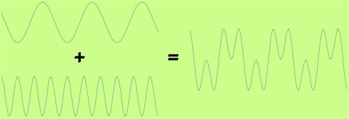
Additive synthesis refers to a number of related synthesis techniques, all based on the idea that complex tones can be created by the summation, or addition, of simpler tones. As we saw in Chapter 3, it is theoretically possible to break up any complex sound into a number of simpler ones, usually in the form of sine waves. In additive synthesis, we use this theory in reverse.

Figure 4.1  Two waves joined by a plus sign.

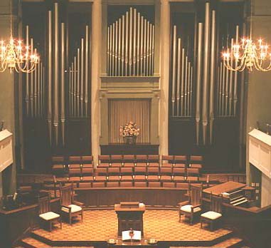
Figure 4.2  This organ has a great many pipes, and together they function exactly like an additive synthesis algorithm.

Each pipe essentially produces a sine wave (or something like it), and by selecting different combinations of harmonically related pipes (as partials), we can create different combinations of sounds, called (on the organ) stops. This is how organs get all those different sounds: organists are experts on Fourier series and additive synthesis (though they may not know that!).

The technique of mixing simple sounds together to get more complex sounds dates back a very long time. In the Middle Ages, huge pipe organs had a great many stops that could be "pulled out" to combine and recombine the sounds from several pipes. In this way, different "patches" could be created for the organ. More recently, the telharmonium, a giant electrical synthesizer from the early 1900s, added together the sounds from dozens of electro-mechanical tone generators to form complex tones. This wasn’t very practical, but it has an important place in the history of electronic and computer music.

Applet 4.2
Mixed sounds

This applet demonstrates how sounds are mixed together.

The Computer and Additive Synthesis

While instruments like the pipe organ were quite effective for some sounds, they were limited by the need for a separate pipe or oscillator for each tone that is being added. Since complex sounds can require anywhere from a couple dozen to several thousand component tones, each needing its own pipe or oscillator, the physical size and complexity of a device capable of producing these sounds would quickly become prohibitive. Enter the computer!

A short excerpt from Kenneth Gaburo’s composition "Lemon Drops," a classic of electronic music made in the early 1960s.

This piece and another extraordinary Gaburo work, "For Harry," were made at the University of Illinois at Urbana-Champaign on an early electronic music instrument called the harmonic tone generator, which allowed the composer to set the frequencies and amplitudes of a number of sine wave oscillators to make their own timbres. It was extremely cumbersome to use, but it was essentially a giant Fourier synthesizer, and, theoretically, any periodic waveform was possible on it!

It’s a tribute to Gaburo’s genius and that of other early electronic music pioneers that they were able to produce such interesting music on such primitive instruments. Kind of makes it seem like we’re almost cheating, with all our fancy software!

If there is one thing computers are good at, it’s adding things together. By using digital oscillators instead of actual physical devices, a computer can add up any number of simple sounds to create extremely complex waveforms. Only the speed and power of the computer limit the number and complexity of the waveforms. Modern systems can easily generate and mix thousands of sine waves in real time. This makes additive synthesis a powerful and versatile performance and synthesis tool. Additive synthesis is not used so much anymore (there are a great many other, more efficient techniques for getting complex sounds), but it’s definitely a good thing to know about.

A Simple Additive Synthesis Sound

Figure 4.3

Let’s design a simple sound with additive synthesis. A nice example is the generation of a square wave.

You can probably imagine what a square wave would look like. We start with just one sine wave, called the fundamental. Then we start adding odd partials to the fundamental, the amplitudes of which are inversely proportional to their partial number. That means that the third partial is 1/3 as strong as the first, the fifth partial is 1/5 as strong, and so on. (Remember that the fundamental is the first partial; we could also call it the first harmonic.) Figure 4.3 shows what we get after adding seven harmonics. Looks pretty square, doesn’t it?

Now, we should admit that there’s an easier way to synthesize square waves: just flip from a high sample value to a low sample value every n samples. The lower the value of n, the higher the frequency of the square wave that’s being generated. Although this technique is clearer and easier to understand, it has its problems too; directly generating waveforms in this way can cause unwanted frequency aliasing.

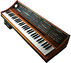
Figure 4.4 The Synclavier was an early digital electronic music instrument that used a large oscillator bank for additive synthesis. You can see this on the front panel of the instrument—many of the LEDs indicate specific partials! On the Synclavier (as was the case with a number of other analog and digital instruments), the user can tune the partials, make them louder, even put envelopes on each one.

Applet 4.3
Additive synthesis

This applet lets you add sine waves together at various amplitudes, to see how additive synthesis works.

Xtra bit 4.4
Spectral formula of a waveform

A More Interesting Example

OK, now how about a more interesting example of additive synthesis? The quality of a synthesized sound can often be improved by varying its parameters (partial frequencies, amplitudes, and envelope) over time. In fact, time-variant parameters are essential for any kind of "lifelike" sound, since all naturally occurring sounds vary to some extent.

These soundfiles are examples of sentences reconstructed with sine waves. Soundfile 4.2 is the sine wave version of the sentence spoken in Soundfile 4.3, and Soundfile 4.4 is the sine wave version of the sentence spoken in Soundfile 4.5.

Sine wave speech is an experimental technique that tries to simulate speech with just a few sine waves, in a kind of primitive additive synthesis. The idea is to pick the sine waves (frequencies and amplitudes) carefully. It’s an interesting notion, because sine waves are pretty easy to generate, so if we can get close to "natural" speech with just a few of them, it follows that we don’t require that much information when we listen to speech.

Sine wave speech has long been a popular idea for experimentation by psychologists and researchers. It teaches us a lot about speech—what’s important in it, both perceptually and acoustically.

These files are used with the permission of Philip Rubin, Robert Remez,
and Haskins Laboratories.

Attacks, Decays, and Time Evolution in Sounds

As we’ve said, additive synthesis is an important tool, and we can do a lot with it. It does, however, have its drawbacks. One serious problem is that while it’s good for periodic sounds, it doesn’t do as well with noisy or chaotic ones.

For instance, creating the steady-state part (the sustain) of a flute note is simple with additive synthesis (just a couple of sine waves), but creating the attack portion of the note, where there is a lot of breath noise, is nearly impossible. For that, we have to synthesize a lot of different kinds of information: noise, attack transients, and so on.

And there’s a worse problem that we’d love to sweep under the old psychoacoustical rug, too, but we can’t: it’s great that we know so much about steady-state, periodic, Fourier-analyzable sounds, but from a cognitive and perceptual point of view, we really couldn’t care less about them! The ear and brain are much more interested in things like attacks, decays, and changes over time in a sound (modulation). That’s bad news for all that additive synthesis software, which doesn’t handle such things very well.

That’s not to say that if we play a triangle wave and a sawtooth wave, we couldn’t tell them apart; we certainly could. But that really doesn’t do us much good in most circumstances. If angry lions roared in square waves, and cute cuddly puppy dogs barked in triangle waves, maybe this would be useful, but we have evolved—or learned to hear attacks, decays, and other transients as being more crucial. What we need to be able to synthesize are transients, spectral evolutions, and modulations. Additive synthesis is not really the best technique for those.

Another problem is that additive synthesis is very computationally expensive. It’s a lot of work to add all those sine waves together for each output sample of sound! Compared to some other synthesis methods, such as frequency modulation (FM) synthesis, additive synthesis needs lots of computing power to generate relatively simple sounds.

But despite its drawbacks, additive synthesis is conceptually simple, and it corresponds very closely to what we know about how sounds are constructed mathematically. For this reason it’s been historically important in computer sound synthesis.

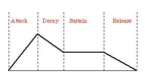
Figure 4.5  A typical ADSR (attack, decay, sustain, release) steady-state modulation. This is a standard amplitude envelope shape used in sound synthesis.

The ability to change a sound’s amplitude envelope over time plays an important part in the perceived "naturalness" of the sound.

Shepard Tones

One cool use of additive synthesis is in the generation of a very interesting phenomenon called Shepard tones. Sometimes called "endless glissandi," Shepard tones are created by specially configured sets of oscillators that add their tones together to create what we might call a constantly rising tone. Certainly the Shepard tone phenomenon is one of the more interesting topics in additive synthesis.

In the 1960s, experimental psychologist Roger Shepard, along with composers James Tenney and Jean-Claude Risset, began working with a phenomenon that scientifically demonstrates an independent dimension in pitch perception called chroma, confirming the circularity of relative pitch judgments.

What circularity means is that pitch is perceived in kind of a circular way: it keeps going up until it hits an octave, and then it sort of starts over again. You might say pitch wraps around (think of a piano, where the C notes are evenly spaced all the way up and down). By chroma, we mean an aspect of pitch perception in which we group together the same pitches that are related as frequencies by multiples of 2. These are an octave apart. In other words, 55 Hz is the same chroma as 110 Hz as 220 Hz as 440 Hz as 880 Hz. It’s not exactly clear whether this is "hard-wired" or learned, or ultimately how important it is, but it’s an extraordinary idea and an interesting aural illusion.

We can construct such a circular series of pitches in a laboratory setting using synthesized Shepard tones. These complex tones are comprised of partials separated by octaves. They are complex tones where all the non-power-of-two numbered partials are omitted.

These tones slide gradually from the bottom of the frequency range to the top. The amplitudes of the component frequencies follow a bell-shaped spectral envelope (see Figure 4.6) with a maximum near the middle of the standard musical range. In other words, they fade in and out as they get into the most common frequency range. This creates an interesting illusion: a circular Shepard tone scale can be created that varies only in tone chroma and collapses the second dimension of tone height by combining all octaves. In other words, what you hear is a continuous pitch change through one octave, but not bigger than one octave (that’s a result of the special spectra and the amplitude curve). It’s kind of like a barber pole: the pitches sound as if they just go around for a while, and then they’re back to where they started (even though, actually, they’re continuing to rise!).

Figure 4.10  Bell-shaped spectral envelope for making Shepard tones.

Shepard wrote a famous paper in 1964 in which he explains, to some extent, our notion of octave equivalence using this auditory illusion: a sequence of these Shepard tones that shifts only in chroma as it is played. The apparent fundamental frequency increases step by step, through repeated cycles. Listeners hear the pitch steps as climbing continuously upward, even though the pitches are actually moving only around the chroma circle. Absolute pitch height (that is, how "high" or "low" it sounds) is removed from our perception of the sequence.

Soundfile 4.6
Shepard tone

Figure 4.7 Try clicking on Soundfile 4.6. After you listen to the soundfile once, click again to listen to the frequencies continue on their upward spiral.

Used with permission from Susan R. Perry, M.A., Dept. of Psychology, University of Tennessee.

Soundfile 4.7
Shepard tone

The Shepard tone contains a large amount of octave-related harmonics across the frequency spectrum, all of which rise (or fall) together. The harmonics toward the low and high ends of the spectrum are attenuated gradually, while those in the middle have maximum amplification. This creates a spiraling or barber pole effect. (Information from Doepfer Musikelektronik GmbH.)

Soundfile 4.7 is an example of the spiraling Shepard tone effect.

Soundfile 4.8
"For Ann" (rising), by James Tenney.

James Tenney is an important computer music composer and pioneer who worked at Bell Laboratories with Roger Shepard in the early 1960s.

This piece was composed in 1969. This composition is based on a set of continuously rising tones, similar to the effect created by Shepard tones. The compositional process is simple: each glissando, separated by some fixed time interval, fades in from its lowest note and fades out as it nears the top of its audible range. It is nearly impossible to follow, aurally, the path of any given glissando, so the effect is that the individual tones never reach their highest pitch.