<-- Back to Previous Page	TOC	Next Section -->

Chapter 3: The Frequency Domain

Section 3.4: The DFT, FFT, and IFFT

The most common tools used to perform Fourier analysis and synthesis are called the fast Fourier transform (FFT) and the inverse fast Fourier transform (IFFT). The FFT and IFFT are optimized (very fast) computer-based algorithms that perform a generalized mathematical process called the discrete Fourier transform (DFT). The DFT is the actual mathematical transformation that the data go through when converted from one domain to another (time to frequency). Basically, the DFT is just a slow version of the FFT—too slow for our impatient ears and brains!

FFTs, IFFTs, and DFTs became really important to a lot of disciplines when engineers figured out how to take samples quickly enough to generate enough data to re-create sound and other analog phenomena digitally. Remember, they don’t just work on sounds; they work on any continuous signal (images, radio waves, seismographic data, etc.).

Xtra bit 3.2
Dan’s history
of the FFT

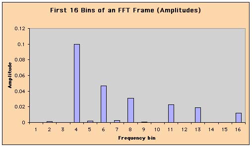
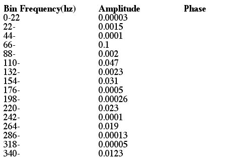
An FFT of a time domain signal takes the samples and gives us a new set of numbers representing the frequencies, amplitudes, and phases of the sine waves that make up the sound we’ve analyzed. It is these data that are displayed in the sonograms we looked at in Section 1.2.

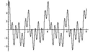
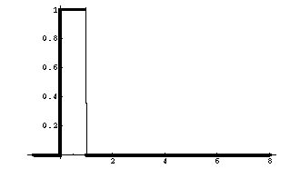
Figure 3.23 Graph and table of spectral components.

Figure 3.23 shows the first 16 bins of a typical FFT analysis after the conversion is made from real and imaginary numbers to amplitude/phase pairs. We left out the phases, because, well, it was too much trouble to just make up a bunch of arbitrary phases between 0 and 2. In a lot of cases, you might not need them (and in a lot of cases, you would!). In this case, the sample rate is 44.1 kHz and the FFT size is 1,024, so the bin width (in frequency) is the Nyquist frequency (44,100/2 = 22,050) divided by the FFT size, or about 22 Hz.

Amplitude values are assumed to be between 0 and 1, and notice that they’re quite small because they all must sum to 1 (and there are a lot of bins!).

We confess that we just sort of made up the numbers; but notice that we made them up to represent a sound that has a simple, more or less harmonic structure with a fundamental somewhere in the 66 Hz to 88 Hz range (you can see its harmonics at around 2, 3, 4, 5, and 6 times its frequency, and note that the harmonics decrease in amplitude more or less like they would in a sawtooth wave).

How the FFT Works

The way the FFT works is fairly straightforward. It takes a chunk of time called a frame (a certain number of samples) and considers that chunk to be a single period of a repeating waveform. The reason that this works is that most sounds are "locally stationary"; meaning that over any short period of time, the sound really does look like a regularly repeating function.

The following is a way to consider this mathematically—taking a window over some portion of some signal that we want to consider as a periodic function.

The Fast Fourier Transform in a Nutshell:
Computing Fourier Coefficients

Here’s a little three-step procedure for digital sound processing.

Window
Periodicize
Fourier transform (this also requires sampling, at a rate equal to 2 times the highest frequency required). We do this with the FFT. Following is an illustration of steps 1 and 2.

Here’s the graph of a (periodic) function, f(t). (Note that f(t) need not be a periodic function.)

Figure 3.24

Suppose we’re only interested in the portion of the graph between 0 ≤ t ≤ 1. Following is a graph of the window function we need to use. We’ll call the function w(t). Note that w(t) equals 1 only in the interval 0 ≤ t ≤ 1 and it’s 0 everywhere else.

Figure 3.25

In step 1, we need to window the function. In Figure 3.25 we’ve plotted both the window function, w(t) (which is nonzero in the region we’re interested in) and function f(t) in the same picture.

Figure 3.26

In Figure 3.26 we’ve plotted f(t)*w(t), which is the periodic function multiplied by the windowing function. From this figure, it’s obvious what part of f(t) we’re interested in.

Figure 3.27

In step 2, we need to periodically extend the windowed function, f(t)*w(t), all along the t-axis.

Figure 3.28

Great! We now have a periodic function, and the Fourier theorem says we can represent this function as a sum of sines and cosines. This is step 3.

Remember, we can also use other, nonsquare windows. This is done to ameliorate the effect of the square windows on the frequency content of the original signal.

Now, once we’ve got a periodic function, all we need to do is figure out, using the FFT, what the component sine waves of that waveform are.

As we’ve seen, it is possible to represent any periodic waveform as a sum of phase-shifted sine waves. In theory, the number of component sine waves is infinite—there is no limit to how many frequency components a sound might have. In practice, we need to limit ourselves to some predetermined number. This limit has a serious effect on the accuracy of our analysis.

Here’s how that works: rather than looking for the frequency content of the sound at all possible frequencies (an infinitely large number—100.000000001 Hz, 100.000000002 Hz, 100.000000003 Hz, etc.), we divide up the frequency spectrum into a number of frequency bands and call them bins. The size of these bins is determined by the number of samples in our analysis frame (the chunk of time mentioned above). The number of bins is given by the formula:

number of bins = frame size/2

Frame Size

So let’s say that we decide on a frame size of 1,024 samples. This is a common choice because most FFT algorithms in use for sound processing require a number of samples that is a power of two, and it’s important not to get too much or too little of the sound.

A frame size of 1,024 samples gives us 512 frequency bands. If we assume that we’re using a sample rate of 44.1 kHz, we know that we have a frequency range (remember the Nyquist theorem) of 0 kHz to 22.05 kHz. To find out how wide each of our frequency bins is, we use the following formula:

bin width = frequency/number of bins

This formula gives us a bin width of about 43 Hz. Remember that frequency perception is logarithmic, so 43 Hz gives us worse resolution at the low frequencies and better resolution at higher frequencies.

By selecting a certain frame size and its corresponding bandwidth, we avoid the problem of having to compute an infinite number of frequency components in a sound. Instead, we just compute one component for each frequency band.

Software That Uses the FFT

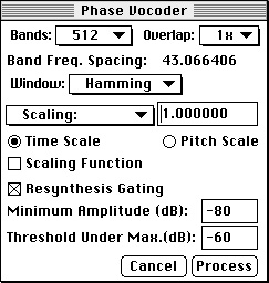
Figure 3.29 Example of a commonly used FFT-based program: the phase vocoder menu from Tom Erbe’s SoundHack.

Note that the user is allowed to select (among several other parameters) the number of bands in the analysis. This means that the user can customize what is called the time/frequency resolution trade-off of the FFT. Don’t ask us what the other options on this screen are—download the program and try it yourself!

There are many software packages available that will do FFTs and IFFTs of your data for you and then let you mess around with the frequency content of a sound. In Chapter 4 we’ll talk about some of the many strange and wonderful things that can be done to a sound in the frequency domain.

Xtra bit 3.3
The mathematics
of magnitude and phase in the FFT

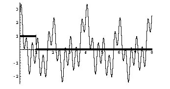
The details of how the FFT works are well beyond the scope of this book. What is important for our purposes is that you understand the general idea of analyzing a sound by breaking it into its frequency components and, conversely, by using a bunch of frequency components to synthesize a new sound. The FFT has been understood for a long time now, and most computer music platforms have tools for Fourier analysis and synthesis.

Figure 3.30 Another way to look at the frequency spectrum is to remove time as an axis and just consider a sound as a histogram of frequencies. Think of this as averaging the frequencies over a long time interval. This kind of picture (where there’s no time axis) is useful for looking at a short-term snapshot of a sound (often just one frame), or perhaps even for trying to examine the spectral features of a sound that doesn’t change much over time (because all we see are the "averages").

The y-axis tells us the amplitude of each component frequency. Since we’re looking at just one frame of an FFT, we usually assume a periodic, unchanging signal. A histogram is generally most useful for investigating the steady-state portion of a sound. (Figure 3.30 is a screen grab from SoundHack.)