|
| <-- Back to Previous Page | TOC | Next Section --> |
Chapter 3: The Frequency DomainSection 3.2: Phasors
|
||
In Chapter 1 we talked about the basic atoms of sound—the sine wave, and about the function that describes the sound generated by a vibrating tuning fork. In this chapter we’re talking a lot about the frequency domain. If you remember, our basic units, sine waves, only had two parameters: amplitude and frequency. It turns out that these dull little sine waves are going to give us the fundamental tool for the analysis and description of sound, and especially for the digital manipulation of sound. That’s the frequency domain: a place where lots of little sine waves are our best friends. But before we go too far, it’s important to fully understand what a sine wave is, and it’s also wonderful to know that we can make these simple little curves ridiculously complicated, too. And it’s useful to have another model for generating these functions. That model is called a phasor. Description of a PhasorThink of a bicycle wheel suspended at its hub. We’re going to paint one of the spokes bright red, and at the end of the spoke we’ll put a red arrow. We now put some axes around the wheel—the x-axis going horizontally through the hub, and the y-axis going vertically. We’re interested in the height of the arrowhead relative to the x-axis as the wheel—our phasor—spins around counterclockwise. |
||
|
Figure 3.7 Sine waves and phasors. As the sine wave moves forward in time, the arrow goes around the circle at the same rate. The height of the arrow (that is, how far it is above or below the x-axis) as it spins around in a circle is described by the sine wave.
Figure 3.8 Phase as angle.
Figure 3.9 Phasor: circle to sine. As time goes on, the phasor goes round and round. At each instant, we measure the height of the dot over the x-axis. Let’s consider a small example first. Suppose the wheel is spinning at a rate of one revolution per second. This is its frequency (and remember, this means that the period is 1 second/revolution). This is the same as saying that the phasor spins at a rate of 360 degrees per second, or better yet, 2\2 This means that after 0.25 second the phasor has gone
Now, let’s look at the function given by the height of the arrow as time goes on. The first thing that we need to remember is a little trigonometry.
This means that:
We’ll make use of this in a minute, because in this example a is the height of our triangle. Similarly, the cosine, written cos(
This means that:
This will come in handy later, too. Now back to our phasor. We’re interested in measuring the height at time t, which we’ll denote as h(t). At time t, the phasor’s arrow is making an angle of
We also get this nice graph of a function, which is our favorite old sine curve.
Figure 3.10 Basic sinusoid. |
||
|
|
||
|
|
This applet traces out a sine curve as a phasor wraps around. |
|
|
|
||
|
|
Then we get this nice curve, which is another kind of sinusoid (bigger!).
Figure 3.11 Bigger sine curve. Now let’s start messing with the frequency, which is the rate of revolution of the phasor. Let’s ramp it up a notch and instead start spinning at a rate of five revolutions per second. Now:
This is easy to see since after 1 second we will have gone five revolutions, which is a total of 10
Now we get this sinusoid:
Figure 3.12 Bigger, faster sine curve. In general, if our phasor is moving at a frequency of
Now we’re almost done, but there is one last thing we could vary: we could change the place where we start our phasor spinning. For example, we could start the phasor moving at a rate of five revolutions per second with a radius of 3, but start the phasor at an angle of Now, what kind of function would this be? Well, at time t = 0 we want to be taking the measurement when the phasor is at an angle of
Figure 3.13 Changing the phase.
Our most general sinusoid of amplitude A, frequency
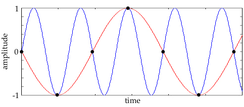
A particularly interesting example is what happens when we take the phase shift equal to 90 degrees, or
Figure 3.14 90-degree phase shift (cosine). You can do some checking on your own and see that this is also the graph that you would get if you plotted the displacement of the arrow from the y-axis. So now we know that a cosine is a phase-shifted sine!
Adding PhasorsFourier’s theorem tells us that any periodic function can be expressed as a sum (possibly with an infinite number of terms!) of sinusoids. (We’ll discuss Fourier’s theorem more in depth later.) Remember, a periodic function is any function that looks like the infinite repetition of some fixed pattern. The length of that basic pattern is called the period of the function. We’ve seen a lot of examples of these in Chapter 1. In particular, if the function has period T, then this sum looks like:
If T is the period of our periodic function, then we now know that its frequency is 1/T—this is also called the fundamental (frequency) of the periodic function, and we see that all other frequencies that occur (called the partials) are simply integer multiples of the fundamental. If you read other books on acoustics and DSP, you will find that partials are sometimes called overtones (from an old German word, "übertonen") and harmonics. There’s often confusion about whether the first overtone is the second partial, and so on. So, to be specific, and also to be more in keeping with modern terminology, we’re always going to call the first partial the one with the frequency of the fundamental. Example: Suppose we have a triangle wave that repeats once every 1/100 second. Then the corresponding fundamental frequency is 100 Hz (it repeats 100 times per second). Triangle waves only contain partials at odd multiples of the fundamental. (The even multiples have no energy—in fact, this is generally true of wave shapes that have the "odd" symmetry, like the triangle wave.) Click on Applet 3.2 and see a triangle wave built by adding one partial after another. |
|
|
|
||
|
|
Building a sawtooth wave partial by partial. |
|
|
|
||
|
|
How should we define an arithmetic of arrows? It sounds funny, but in fact it’s a pretty natural generalization of what we already know about adding regular old numbers. When we add a negative number, we go backward, and when we add a positive number, we go forward. Our regular old numbers can be thought of as arrows on a number line. Adding any two numbers, then, simply means taking the two corresponding arrows and placing them one after the other, tip to tail. The sum is then the arrow from the origin pointing to the place where "adding" the two arrows landed you. Really, what we are doing here is thinking of numbers as vectors. They have a magnitude (length) and a direction (in this case, positive or negative, or better yet 0 radians or Now, to add phasors, we need to enlarge our worldview and allow our arrows to get not just 2 directions, but instead a whole 2 So, to recap: to add phasors, at each instant as our phasors are spinning around, we add the two arrows. In this way, we get a new arrow spinning around (the sum) at some frequency—a new phasor. Now it’s easy to see that the sum of two phasors of the same frequency yields a new phasor of the same frequency. We can also see that the sum of a cosine and sine of the same frequency is simply a phase-shifted sine of the same frequency with a new amplitude given by the square root of the sum of squares of the two original phasors. That’s the Pythagorean theorem! Sampling and Fourier Expansion
Figure 3.15 The decomposition of a complex waveform into its component phasors (which is pretty much the same as saying the decomposition of an acoustic waveform into its component partials) is called Fourier expansion. In practice, the main thing that happens is that analog waveforms are sampled, creating a time-domain representation inside the computer. These samples are then converted (using what is called a fast Fourier transform, or FFT) into what are called Fourier coefficients.
Figure 3.16 FFT of sampled phasors exp(2*j*
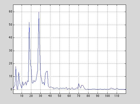
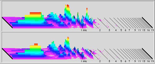
Figure 3.17 FFT plot of a gamelan instrument. Figure 3.17 shows a common way to show timbral information, especially the way that harmonics add up to produce a waveform. However, it can be slightly confusing. By running an FFT on a small time-slice of the sound, the FFT algorithm gives us the energy in various frequency bins. (A bin is a discrete slice, or band, of the frequency spectrum. Bins are explained more fully in Section 3.4.) The x-axis (bottom axis) shows the bin numbers, and the y-axis shows the strength (energy) of each partial. The slightly strange thing to keep in mind about these bins is that they are not based on the frequency of the sound itself, but on the sampling rate. In other words, the bins evenly divide the sampling frequency (linearly, not exponentially, which can be a problem, as we’ll explain later). Also, this plot shows just a short fraction of time of the sound: to make it time-variant, we need a waterfall 3D plot, which shows frequency and amplitude information over a span of time. Although theoretically we could use the FFT data shown in Figure 3.17 in its raw form to make a lovely, synthetic gamelan sound, the complexity and idiosyncracies of the FFT itself make this a bit difficult (unless we simply use the data from the original, but that’s cheating). Figure 3.18 shows a better graphical representation of sound in the frequency domain. Time is running from front to back, height is energy, and the x-axis is frequency. This picture also takes the essentially linear FFT and shows us an exponential image of it, so that most of the "action" happens in the lower 2k, which is correct. (Remember that the FFT divides the frequency spectrum into linear, equal divisions, which is not really how we perceive sound—it’s often better to graph this exponentially so that there’s not as much wasted space "up top.") The waterfall plot in Figure 3.18 is stereo, and each channel of sound has its own slightly different timbre.
Figure 3.18 Waterfall plot. Here’s a fact that will help a great deal: if the highest frequency is B times the fundamental, then you only need 2B + 1 samples to determine the Fourier coefficients. (It’s easy to see that you should need at least 2B, since you are trying to get 2B pieces of information (B amplitudes and B2 phase shifts).)
Figure 3.19 Aliasing, foldover. This is a phenomenon that happens when we try to sample a frequency that is more than half the sampling rate, or the Nyquist frequency. As the frequency we want to sample gets higher than half the sampling rate, we start "undersampling" and get unwanted, lower-frequency artifacts (that is, low frequencies created by the sampling process itself). |
|
| <-- Back to Previous Page | Next Section --> |
©Burk/Polansky/Repetto/Roberts/Rockmore. All rights reserved.
 The sine and cosine of an angle are measured using a right triangle. For our right triangle, the sine of